18 Performance

Outline

Example performance optimisation workflow
General techniques
Benchmarking by yourself

Recommended Readings:

Workflow:

Have correct implementation
Profile (profvi, microbenchmark)
Optimise

18.1 Good practices

rm(list = ls()) at the beginning of your script
Make sure you understand all warnings
Don’t repeat yourself (DRY)
- Use functions (Session 1)
- Vectorise functions (Session 3)
- Use inheritance (Session 6)
Readable code
- Comment where needed
- No magic numbers
- Variable names
  - BigCamelCase for function names
  - snake_case for everything else
  - ALL_CAPS for constants
- Version control

18.2 Code Profiling

We now demonstrate the process of optimising the performance of an algorithm’s implementation using the profiling tool provided by RStudio. The algorithm we implement is the Monte Carlo integration method to estimate the value of pi. The idea is to randomly sample points in a unit square and count how many of them fall within a quarter circle inscribed within that square. The ratio of points inside the quarter circle to the total number of points sampled can be used to estimate pi.

18.2.1 Version 1

MonteCarloPiV1 <- function (n) {
  stopifnot(n > 1)
  n_inside_count <- 0
  for (ii in seq_len(n)) {
    x <- runif(1)
    y <- runif(1)
    if (x^2 + y^2 < 1) {
      n_inside_count <- n_inside_count + 1
    }
  }
  return(n_inside_count / n)
}

N <- 500000
system.time(pi_est <- MonteCarloPiV1(N)*4)

stopifnot(pi_est - pi < 0.01)
print("test passed")

profvis - Profile an R expression and visualise profiling data
RStudio > Profile > Profile Selected Line(s)
We see that most of the time is spent on the two runif calls

18.2.2 Version 2

MonteCarloPiV2 <- function (n) {
  stopifnot(n > 1)
  n_inside_count <- 0
  x_sq <- runif(n)
  y_sq <- runif(n)
  for (ii in seq_along(x_sq)) {
    if (x_sq[ii]^2 + y_sq[ii]^2 < 1) {
      n_inside_count <- n_inside_count + 1
    }
  }
  return(n_inside_count / n)
}
# MonteCarloPiV2(1000)*4
N <- 500000
N <- N * 10
system.time(pi_est <- MonteCarloPiV2(N)*4)


stopifnot(pi_est - pi < 0.01)
print("test passed")

Increase the size of N to see that most of the time is spent in the for loop

18.2.3 Version 3

MonteCarloPiV3 <- function (n) {
  stopifnot(n > 1)
  n_inside_count <- 0
  x_sq <- runif(n)
  y_sq <- runif(n)
  
  d_sq <- x_sq^2 + y_sq^2
  d_sq_bol <- d_sq < 1
  
  n_inside_count <- length(d_sq_bol[d_sq_bol == TRUE])
  
  return(n_inside_count / n)
}
# MonteCarloPiV2(1000)*4
N <- 500000
N <- N * 10
system.time(pi_est <- MonteCarloPiV3(N)*4)


stopifnot(pi_est - pi < 0.01)
print("test passed")

18.2.4 Version 4

MonteCarloPiV4 <- function (n) {
  stopifnot(n > 1)
  n_inside_count <- 0
  x_sq <- runif(n)
  y_sq <- runif(n)
  
  d_sq <- x_sq^2 + y_sq^2
  d_sq_bol <- d_sq < 1
  
  n_inside_count <- sum(d_sq_bol, na.rm = TRUE)
  
  return(n_inside_count / n)
}
# MonteCarloPiV2(1000)*4
N <- 500000
N <- N * 10
system.time(pi_est <- MonteCarloPiV4(N)*4)


stopifnot(pi_est - pi < 0.01)
print("test passed")

18.2.5 `microbenchmark`

N <- 500000
# N <- N * 10
if (!exists("mb_res1")) {
  mb_res1 <- microbenchmark::microbenchmark(
            times = 100, unit = "ms",
            MonteCarloPiV1(N),
            MonteCarloPiV2(N),
            MonteCarloPiV3(N),
            MonteCarloPiV4(N)              
          )
}

# print(mb_res)
# boxplot(mb_res)

ggplot2::autoplot(mb_res1) #+
  # scale_fill_viridis(discrete=TRUE)

18.3 General principles

18.3.1 Don’t grow your data

rm(list = ls())

Fun1 <- function(n) {
  res <- NULL
  for (ii in seq_len(n)) {
    res <- c(res, ii)
  }
  return(res)
}

Fun2 <- function(n) {
  res <- numeric(n) # pre-allocate memory space
  for (ii in seq_len(n)) {
    res[ii] <- ii
  }
  return(res)
}

Fun3 <- function(n) {
  return(seq_len(n)) # use a built-in function when possible
}

N <- 10000
if (!exists("mb_res2")) {
  mb_res2 <- microbenchmark::microbenchmark(
    times = 100, unit = "ms",
    Fun1(N), Fun2(N), Fun3(N)
  )
}

Warning in microbenchmark::microbenchmark(times = 100, unit = "ms", Fun1(N), :
less accurate nanosecond times to avoid potential integer overflows

ggplot2::autoplot(mb_res2)

Warning: `aes_string()` was deprecated in ggplot2 3.0.0.
ℹ Please use tidy evaluation idioms with `aes()`.
ℹ See also `vignette("ggplot2-in-packages")` for more information.
ℹ The deprecated feature was likely used in the microbenchmark package.
  Please report the issue at
  <https://github.com/joshuaulrich/microbenchmark/issues/>.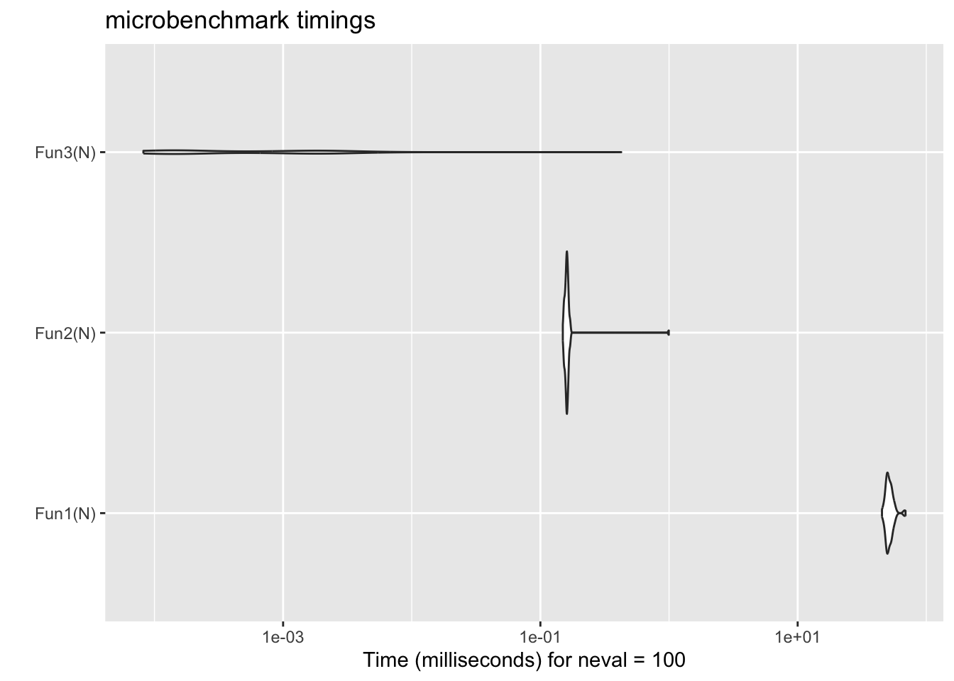

18.3.2 Lazy evaluation

rm(list = ls())

N <- 1e6
V <- runif(N)
v1 <- V > 0.1
v2 <- V > 0.4
v3 <- V > 0.9

mb_res_le <- microbenchmark::microbenchmark(
  times = 100, unit = "ms",
  which(v1 & v2 & v3), which(v3 & v2 & v1)
)
stopifnot(identical(which(v1 & v2 & v3), which(v3 & v2 & v1)))
ggplot2::autoplot(mb_res_le)

mb_res_le_or <- microbenchmark::microbenchmark(
  times = 100, unit = "ms",
  which(v1 | v2 | v3), which(v3 | v2 | v1)
)
stopifnot(identical(which(v1 | v2 | v3), which(v3 | v2 | v1)))
ggplot2::autoplot(mb_res_le_or)

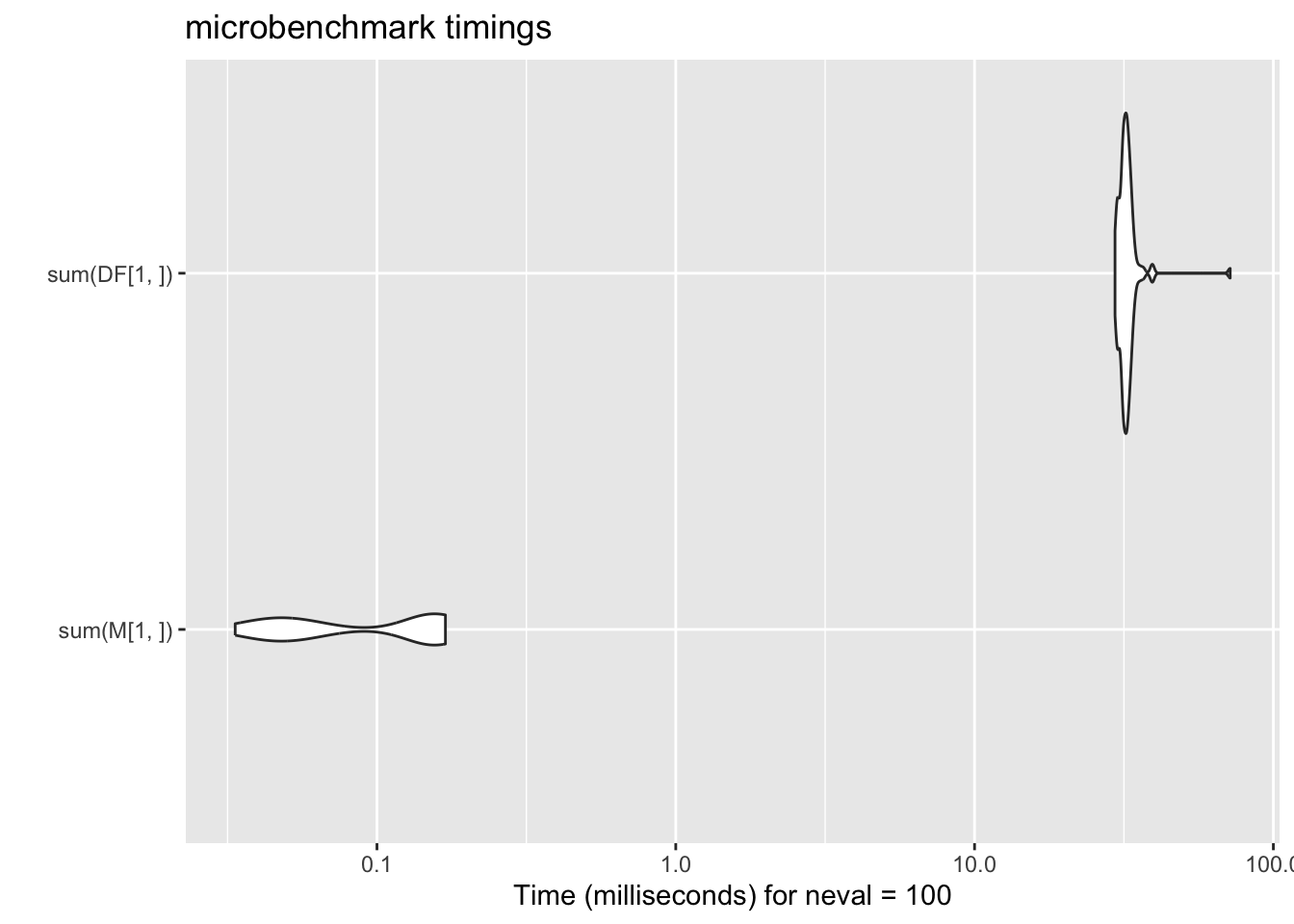
18.3.3 Use low level structure

rm(list = ls())

C <- 10000
M <- matrix(runif(C^2), nrow = C)
DF <- as.data.frame(M)

mb_res4 <- microbenchmark::microbenchmark(
  times = 100, unit = "ms",
  sum(M[1, ]), sum(DF[1, ])
)
stopifnot(sum(M[1, ]) == sum(DF[1, ]))
ggplot2::autoplot(mb_res4)

18.4 BIY

Benchmark it yourself

18.4.1 Check for `NA`

rm(list = ls())

N <- 1e5
V <- runif(N)

V_has_NA_l <- V # low
V_has_NA_m <- V # mid
V_has_NA_h <- V # high


V_has_NA_l[1] <- NA
V_has_NA_m[N/2] <- NA
V_has_NA_h[N] <- NA

mb_res5 <- microbenchmark::microbenchmark(
  times = 100, unit = "ms",
  anyNA(V), any(is.na(V)), is.na(sum(V)),
  anyNA(V_has_NA_l), any(is.na(V_has_NA_l)), is.na(sum(V_has_NA_l)),
  anyNA(V_has_NA_m), any(is.na(V_has_NA_m)), is.na(sum(V_has_NA_m)),
  anyNA(V_has_NA_h), any(is.na(V_has_NA_h)), is.na(sum(V_has_NA_h))
)

Warning in microbenchmark::microbenchmark(times = 100, unit = "ms", anyNA(V), :
Could not measure a positive execution time for 7 evaluations.

stopifnot(!any(
  anyNA(V), any(is.na(V)), is.na(sum(V))
))
stopifnot(all(
  anyNA(V_has_NA_l), any(is.na(V_has_NA_l)), is.na(sum(V_has_NA_l))
))
stopifnot(all(
  anyNA(V_has_NA_m), any(is.na(V_has_NA_m)), is.na(sum(V_has_NA_m))
))
stopifnot(all(
  anyNA(V_has_NA_h), any(is.na(V_has_NA_h)), is.na(sum(V_has_NA_h))
))

library("ggplot2", "RColorBrewer")
# ggplot2::autoplot(mb_res5, fill = expr) +
#   scale_fill_brewer(palette="Set1")

col_list <- c("#E41A1C", "#984EA3", "#4DAF4A") #"#377EB8"

ggplot(data = mb_res5, aes(x = expr, y = time, fill = expr, col = expr)) + 
  geom_violin() + 
  scale_y_continuous(trans = "log10") +
  # scale_fill_brewer(palette="Set1") +
  scale_color_manual(values = rep(col_list, 4)) +
  scale_fill_manual(values = rep(col_list, 4)) +
  theme(legend.position = "none") +
  coord_flip()

Warning in scale_y_continuous(trans = "log10"): log-10 transformation
introduced infinite values.

Warning: Removed 26 rows containing non-finite outside the scale range
(`stat_ydensity()`).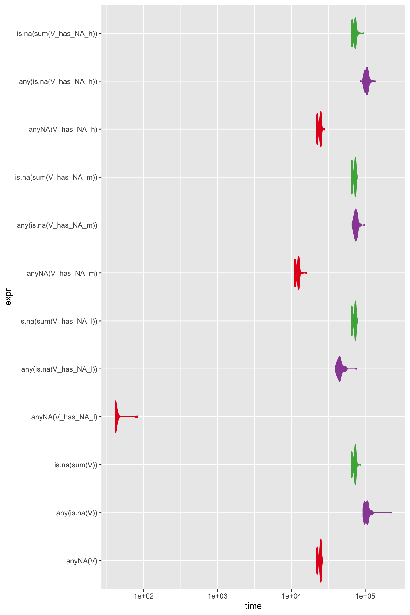

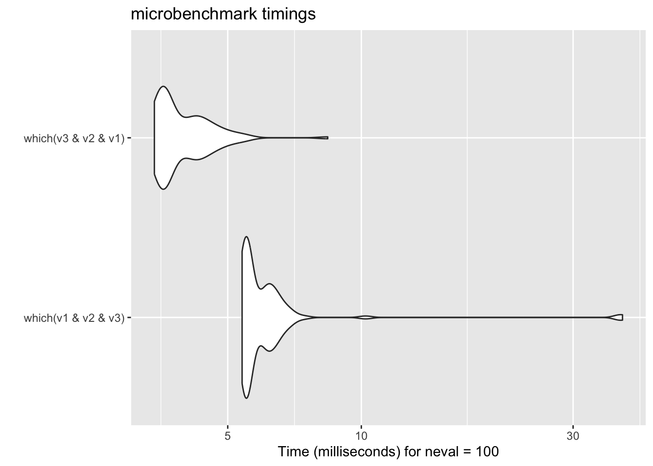
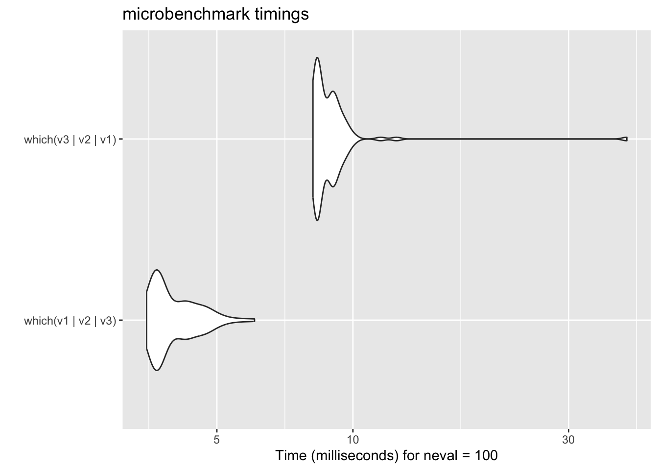
Some algorithms’ performance is data dependent

18.4.2 Column-wise max

rm(list = ls())
C <- 100
# C <- 1000 # Some algorithm's performance is data-dependent
# M <- matrix(1:C^2, nrow = C/2)
M <- matrix(runif(C^2), nrow = C/2)

Fun1 <- function(m) {
  c <- ncol(m)
  res <- numeric(c)
  
  for (cc in seq_len(c)) {
    res[cc] <- max(m[, cc])
  }
  return(res)
}

Fun1_glb <- function() {
  c <- ncol(M)
  res <- numeric(c)
  for (cc in seq_len(c)) {
    res[cc] <- max(M[, cc])
  }
  return(res)
}
stopifnot(identical(Fun1(M), Fun1_glb()))

Fun2 <- function(m) {
  return(apply(m, MARGIN = 2, max))
}

Fun2_glb <- function() {
  return(apply(M, MARGIN = 2, max))
}
# stopifnot(identical(Fun2(M), Fun2_glb()))

# stopifnot(all.equal(Fun1(M), Fun2(M), matrixStats::colMaxs(M)))


mb_res3 <- microbenchmark::microbenchmark(
  times = 100, unit = "ms",
  Fun1(M),
  Fun1_glb(),
  Fun2(M),
  Fun2_glb,
  apply(M, MARGIN = 2, max),
  matrixStats::colMaxs(M)
)

Warning in microbenchmark::microbenchmark(times = 100, unit = "ms", Fun1(M), :
Could not measure a positive execution time for 26 evaluations.

ggplot2::autoplot(mb_res3)

Warning in ggplot2::scale_y_log10(name = y_label): log-10 transformation
introduced infinite values.

Warning: Removed 67 rows containing non-finite outside the scale range
(`stat_ydensity()`).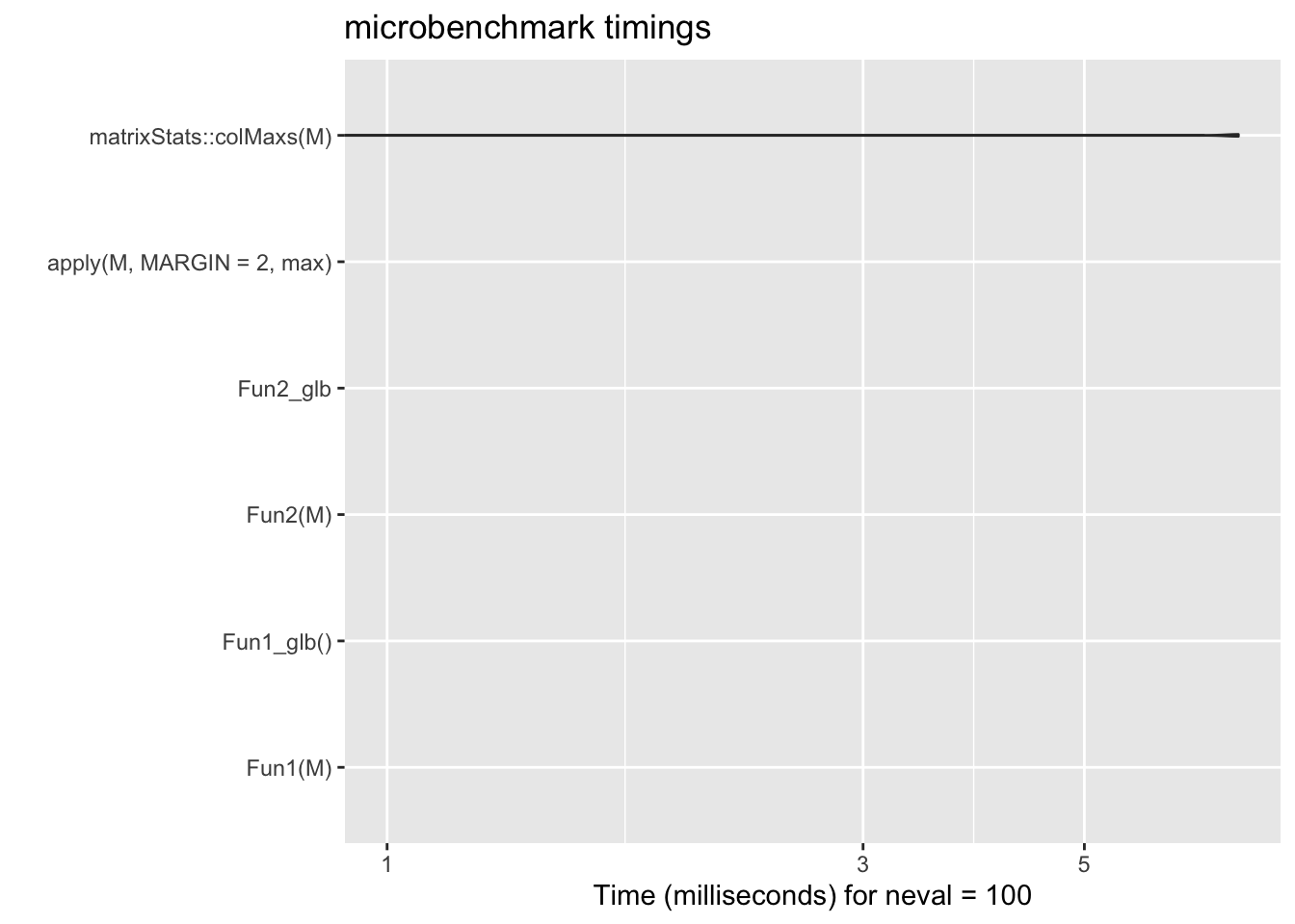

# typeof(M)
# a <- Fun1(M)
# b <- Fun2(M)
# typeof(a)
# typeof(b)
# typeof(matrixStats::colMaxs(M))

18.4.3 Row-wise sum

rm(list = ls())

C <- 1000
# C <- 1000 # Some algorithm's performance is data-dependent
# M <- matrix(1:C^2, nrow = C/2)
M <- matrix(runif(C^2), nrow = C)

# stopifnot(all.equal(
#   apply(M, MARGIN = 1, sum),
#   rowSums(M),
#   matrixStats::rowSums2(M)
# ))

mb_res_sum <- microbenchmark::microbenchmark(
  times = 10, unit = "ms",
  apply(M, MARGIN = 1, sum),
  rowSums(M),
  matrixStats::rowSums2(M)
)
ggplot2::autoplot(mb_res_sum)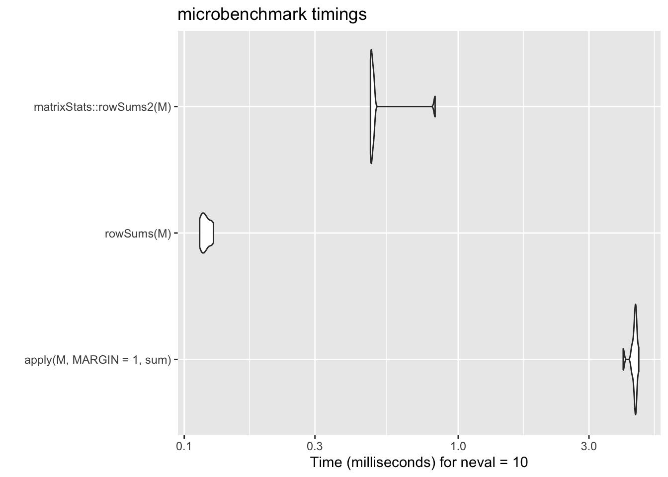

18.5 Summary

Use vectorised function
- Remember that there is no scalar type in R
- Know which functions are vectorised
- Avoid for loop when possible
Hand over to R as soon as possible
Don’t grow your data
Utilise lazy evaluation
Use low level structure
Specify integer when possible
Compare different methods yourself
Ask Google (example)
There is Rcpp to look forward to

Revision

What have we achieved this week:
- We learnt ~5% of what R can do, maybe.
- The CRAN package repository features 18090 packages, source
- We learnt ~0.01% of what programming languages can do, likely less.
What is R?
- Look at the language as a statistician

Top programming languages 2021, IEEE Spectrum

Functions
- Session 1:
  - How to write your own function
  - Everything that happens in R is a function call
- Session 2:
  - Function environment
- Session 3&4:
  - Apply functions to vectors
Vectors
- Session 3
  - There is no scalar type in R
  - Everything is a fancy vector
- Session 4
  - How to work with vectors
- Session 9
  - Utilise vectorised functions

What to do next?

Practice, practice, …
- Project Euler, https://projecteuler.net/
- https://leetcode.com/
- Advanced R Solutions
- Code reading skills
Get help in R
- ?
- str
Learn editor tricks
- ALT + click up/down
- ALT + SHIFT + click and drag a rectangle
- CTRL + ALT + SHIFT + M (find in scope)
- More tricks

Assessment Time