16  Statistical Models

Model building in R

What is R? - R is a language and environment for statistical computing and graphics.

Outline

• Model types
• Statistical methods
  • Linear interpolation
  • Linear regression
  • Nonlinear regression
  • Optimisation
• Mathematical models
  • Model limits
  • Lorenz system
  • Solve differential equations with desolve
  • Exponential growth model
  • Logistic growth model
  • Lotka-Volterra model
  • Drug concentration model

Recommended readings:

• Chapter 23, R for Data Science, Hadley

Model types

WorldPhones is a dataset for the number of telephones in various regions of the world (in thousands) in the 1950s.

WorldPhones

     N.Amer Europe Asia S.Amer Oceania Africa Mid.Amer
1951  45939  21574 2876   1815    1646     89      555
1956  60423  29990 4708   2568    2366   1411      733
1957  64721  32510 5230   2695    2526   1546      773
1958  68484  35218 6662   2845    2691   1663      836
1959  71799  37598 6856   3000    2868   1769      911
1960  76036  40341 8220   3145    3054   1905     1008
1961  79831  43173 9053   3338    3224   2005     1076

We see that data for a few years between 1951 and 1956 are missing.

x_data <- rownames(WorldPhones)[1:2]
y_data <- WorldPhones[1:2, "N.Amer"]
{
plot(
  x = x_data, xlab = "Years (t)", col = "blue", pch = 16,
  y = y_data, ylab = "number of phones (n)"
)
text(x = 1953, y = 52500 + (rnorm(7)*3000), labels = c("?"))
}

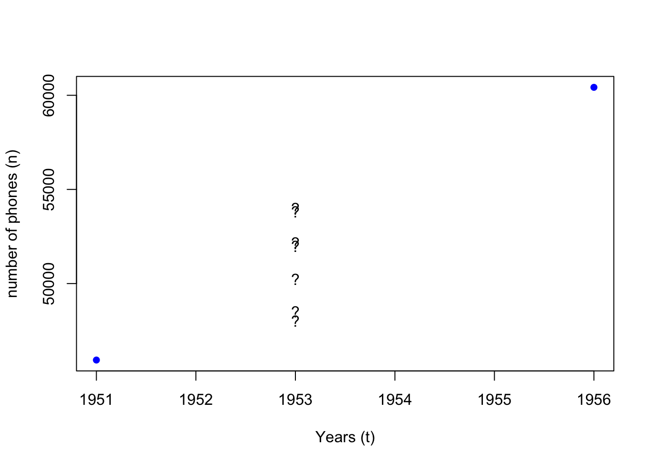
What if we want to estimate how many phones “N.Amer” had in 1953?

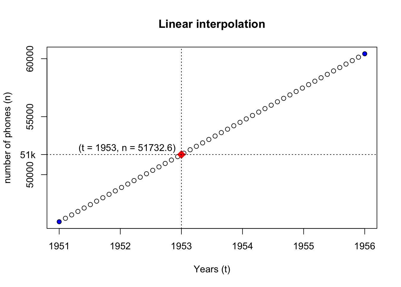
• We assume that the increase in the number of phones (\(n\)) is constant over time (\(t\))
• We assume that the values between 1951 and 1956 are only related to these two data points

---

• Method 1 : Linear interpolation (approx, approxfun)

a <- approx(x = x_data, y = y_data)
afunc <- approxfun(x = x_data, y = y_data)
wanted_t <- 1953
wanted_n <- afunc(wanted_t)

{
plot(
  x = rownames(WorldPhones)[1:2], xlab = "Years (t)", col = "blue", pch = 16,
  y = WorldPhones[1:2, "N.Amer"], ylab = "number of phones (n)",
  main = "Linear interpolation"
)
points(a)
points(x = wanted_t, y = wanted_n, pch = 18, col = "red", cex = 2)
text(x = wanted_t, y = wanted_n * 1.01, labels = paste0("(t = ", wanted_t, ", n = ", wanted_n, ")"), pos = 2)
abline(v = wanted_t, lty = "dotted")
abline(h = wanted_n, lty = "dotted")
axis(2, at = wanted_n, labels = paste0(wanted_n%/%1000, "k"), las = 2)
}

• Method 2 : Mathematical model

dndt <- diff(y_data) / diff(as.numeric(x_data))

YearStep <- function(n_prev_year, dndt) {
  return(n_prev_year + dndt)
}

n <- y_data[1]
num_years <- wanted_t - as.numeric(x_data[1])
stopifnot(num_years >= 1)
for (tt in 1:num_years) {
  n <- YearStep(n, dndt)
}
n
  
# simplified version
# f <- function(init_n, init_t, dndt, t) {
#   return(init_n + (t - init_t) * dndt)
# }
# f(y_data[1], as.numeric(x_data[1]), dndt, wanted_t) 

We see that although the two methods reach the same conclusion, their modelling methods differ.

• Method 1 (statistical): values are interpolated between the two known data points
• Method 2 (mathematical): the yearly rate of change (\(dn/dt\)) is worked out for the state change equation
• The initial assumption that the number of phones (\(n\)) increase linearly in time (\(t\)) is often a conclusion drawn from statistical analysis of the known data points.
• Statistical models build on the premise that a pattern is identifiable from a set of data points, and estimate the probability distribution of a set of outcomes.
• Mathematical models describe the mechanisms of real world event with a set of equations (a system of equations), and derive predictions via simulation.
• Statistics is a mathematical discipline, and statistical models are a special class of mathematical model that uses statistical methods to describe data and make inferences
• Mathematical model, just like mathematics, is widely applied across disciplines.

More on the difference between statistical and mathematical modelling approaches

---

Statistical models

16.1 Interpolation

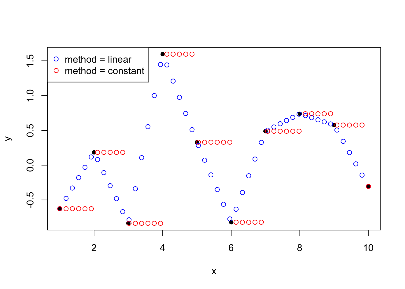
• Linear interpolation
  • approx - returns a list of points which linearly interpolate given data points.
  • approxfun - returns a function that performs the interpolation.
• Polynomial interpolation
  • spline - returns a list of points along the spline interpolation of the given data points.
  • splinefun - returns a function of the spline interpolation

?approx:

• with approx:

set.seed(1)
x <- 1:10
y <- rnorm(10)
{
plot(x, y, pch = 16)
points(approx(x, y), col = "blue")
points(approx(x, y, method = "constant"), col = "red")
legend("topleft",
    legend = c("method = linear", "method = constant"),
    col = c("blue", "red"),
    pch = c(1, 1)
)
}

• approxfun

f <- approxfun(x, y)
{
curve(f(x), 1, 10, col = "green2")
points(x, y)
}

• splinefun

# x <- 1:10
# y <- rnorm(10)
f <- splinefun(x, y)
curve(f(x), 1, 10)
points(x, y)

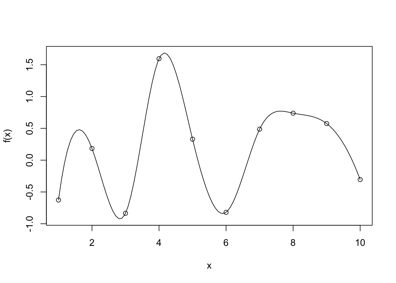
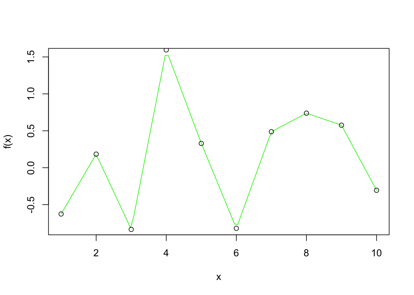
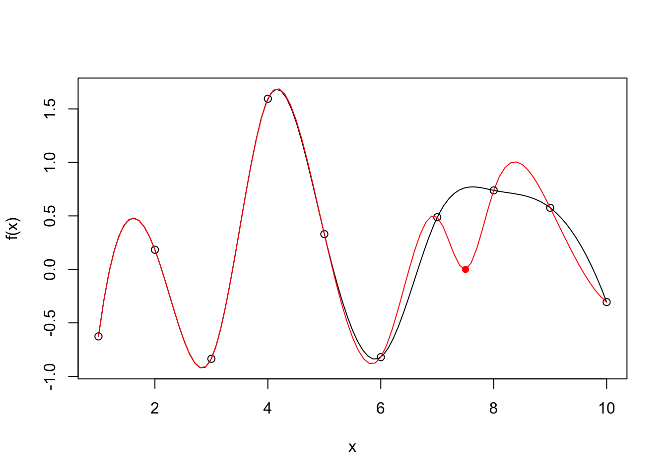
Interpolation methods ensures that the fitted curve goes through every point in the observed dataset. A bit like connecting the dots:

• It is great at preserving the known data exactly
• It preserves all flaws that the data carries
• Selective representation of the real world situation, missing data points are not represented
• Over fit

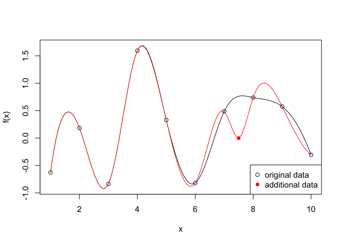
Example:

# x <- 1:10
# y <- rnorm(10)
# f <- splinefun(x, y)
x_extra <- 7.5
y_extra <- 0
f2 <- splinefun(c(x, x_extra), c(y, y_extra))

{
curve(f(x), 1, 10)
points(x, y)
# par(new = TRUE)
x2 <- seq(1, 10, by = 0.1)
y2 <- f2(x2)
lines(x2, y2, col = "red")
points(x_extra, y_extra, col = "red", pch = 16)
legend("bottomright", legend = c("original data", "additional data"), pch = c(1, 16), col = c("black", "red"))
}

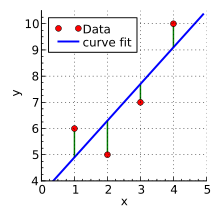
16.2 Linear regression

?lm - performs linear least squares regression to fit linear models

residuals of least square fit, image source

16.2.1 Dobson 2.2.2

This dataset comes from section 2.2.2 of Annette J. Dobson, “An introduction to generalized linear models”, 2nd edition:

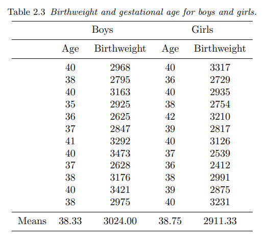
In this table are the birthweights (in grams) and estimated gestational ages (in weeks) of 12 boys and 12 girls born in a certain hospital.

dtf <- data.frame(
  age = c(40, 38, 40, 35, 36, 37, 41, 40, 37, 38, 40, 38,  # boys
          40, 36, 40, 38, 42, 39, 40, 37, 36, 38, 39, 40), # girls

  weight = c(2968, 2795, 3163, 2925, 2625, 2847, 3292, 3473, 2628, 3176, 3421, 2975, # boys
             3317, 2729, 2935, 2754, 3210, 2817, 3126, 2539, 2412, 2991, 2875, 3231), # girls

  gender = gl(2, 12, 24, labels = c("boys", "girls"))
)
summary(dtf)

      age            weight       gender  
 Min.   :35.00   Min.   :2412   boys :12  
 1st Qu.:37.00   1st Qu.:2785   girls:12  
 Median :38.50   Median :2952             
 Mean   :38.54   Mean   :2968             
 3rd Qu.:40.00   3rd Qu.:3184             
 Max.   :42.00   Max.   :3473             

Let’s use the simple weight is a function of age formula:

f1 <- weight ~ age
lm1 <- lm(f1, data = dtf)
summary(lm1)

Call:
lm(formula = f1, data = dtf)

Residuals:
    Min      1Q  Median      3Q     Max 
-262.03 -158.29    8.35   88.15  366.50 

Coefficients:
            Estimate Std. Error t value Pr(>|t|)    
(Intercept)  -1485.0      852.6  -1.742   0.0955 .  
age            115.5       22.1   5.228 3.04e-05 ***
---
Signif. codes:  0 '***' 0.001 '**' 0.01 '*' 0.05 '.' 0.1 ' ' 1

Residual standard error: 192.6 on 22 degrees of freedom
Multiple R-squared:  0.554, Adjusted R-squared:  0.5338 
F-statistic: 27.33 on 1 and 22 DF,  p-value: 3.04e-05

• The R-squared values is between 0 and 1. The lower end (closer to 0) indicate a poorly fitted model, the higher end (closer to 1) indicate a model of good fit.
• A p-value that’s less than 0.05 means an independent variable (predictor) plays a meaningful part in the fitted model.
• A small p-value of 3.04e-05 means that age plays a significant part in this model.
• A p-value of 0.0955 means that the intercept term is not significant for this model.

Let’s take a look at the coefficients of the fitted model:

attributes(lm1)

$names
 [1] "coefficients"  "residuals"     "effects"       "rank"         
 [5] "fitted.values" "assign"        "qr"            "df.residual"  
 [9] "xlevels"       "call"          "terms"         "model"        

$class
[1] "lm"

lm1$coefficients

(Intercept)         age 
 -1484.9846    115.5283 

The fitted formula is \(weight = -1484.9846 + 115.5283\times age\):

{
plot(f1, data = dtf,  xlim = c(0,42), ylim = c(-1500, 3400))
abline(lm1, col = "red")
abline(h = 0)
}#plot(lm1)

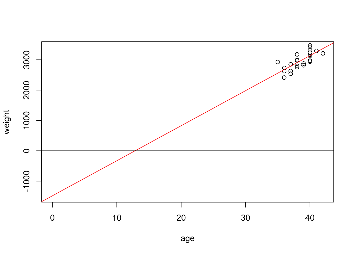
• The negative intercept means that the baby has a negative weight at age 0

predict(object = lm1, newdata = data.frame(age = 0)) # weight when age is 0 (intercept)

        1 
-1484.985 

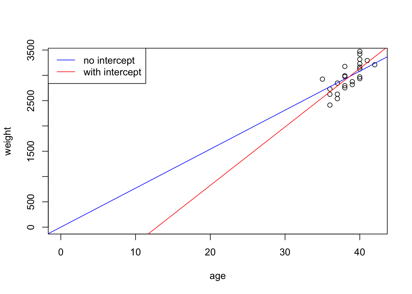
Let’s drop the intercept term from the formula:

f2 <- weight ~ age - 1
lm2 <- lm(f2, data = dtf)
summary(lm2)

Call:
lm(formula = f2, data = dtf)

Residuals:
    Min      1Q  Median      3Q     Max 
-362.91 -148.65  -16.19  135.71  389.77 

Coefficients:
    Estimate Std. Error t value Pr(>|t|)    
age   77.081      1.063   72.51   <2e-16 ***
---
Signif. codes:  0 '***' 0.001 '**' 0.01 '*' 0.05 '.' 0.1 ' ' 1

Residual standard error: 200.9 on 23 degrees of freedom
Multiple R-squared:  0.9956,    Adjusted R-squared:  0.9955 
F-statistic:  5258 on 1 and 23 DF,  p-value: < 2.2e-16

The p-value for age is 2.2e-16. Compare the two fitted models:

{
plot(f2, data = dtf, xlim = c(0,42), ylim = c(0, 3400))
abline(lm2, col = "blue")
abline(lm1, col = "red")
legend("topleft", c("no intercept", "with intercept"), lty = 1, col = c("blue", "red"))
}

---

We can bring gender into the formula:

f3 <- weight ~ 0 + age + gender
lm3 <- lm(f3, data = dtf)
summary(lm3)

Call:
lm(formula = f3, data = dtf)

Residuals:
    Min      1Q  Median      3Q     Max 
-257.49 -125.28  -58.44  169.00  303.98 

Coefficients:
            Estimate Std. Error t value Pr(>|t|)    
age           120.89      20.46   5.908 7.28e-06 ***
genderboys  -1610.28     786.08  -2.049   0.0532 .  
gendergirls -1773.32     794.59  -2.232   0.0367 *  
---
Signif. codes:  0 '***' 0.001 '**' 0.01 '*' 0.05 '.' 0.1 ' ' 1

Residual standard error: 177.1 on 21 degrees of freedom
Multiple R-squared:  0.9969,    Adjusted R-squared:  0.9965 
F-statistic:  2258 on 3 and 21 DF,  p-value: < 2.2e-16

---

We can also fit the two genders separately:

lm2_boys <- lm(f2, data = dtf, subset = (gender == "boys"))
lm2_girls <- lm(f2, data = dtf, subset = (gender == "girls"))
summary(lm2_boys)

Call:
lm(formula = f2, data = dtf, subset = (gender == "boys"))

Residuals:
    Min      1Q  Median      3Q     Max 
-293.50 -194.15  -10.41  164.95  314.62 

Coefficients:
    Estimate Std. Error t value Pr(>|t|)    
age   78.959      1.515   52.13 1.59e-14 ***
---
Signif. codes:  0 '***' 0.001 '**' 0.01 '*' 0.05 '.' 0.1 ' ' 1

Residual standard error: 201.3 on 11 degrees of freedom
Multiple R-squared:  0.996, Adjusted R-squared:  0.9956 
F-statistic:  2718 on 1 and 11 DF,  p-value: 1.593e-14

summary(lm2_girls)

Call:
lm(formula = f2, data = dtf, subset = (gender == "girls"))

Residuals:
    Min      1Q  Median      3Q     Max 
-296.72 -108.26  -19.58  120.19  307.31 

Coefficients:
    Estimate Std. Error t value Pr(>|t|)    
age   75.242      1.345   55.95 7.34e-15 ***
---
Signif. codes:  0 '***' 0.001 '**' 0.01 '*' 0.05 '.' 0.1 ' ' 1

Residual standard error: 180.7 on 11 degrees of freedom
Multiple R-squared:  0.9965,    Adjusted R-squared:  0.9962 
F-statistic:  3130 on 1 and 11 DF,  p-value: 7.343e-15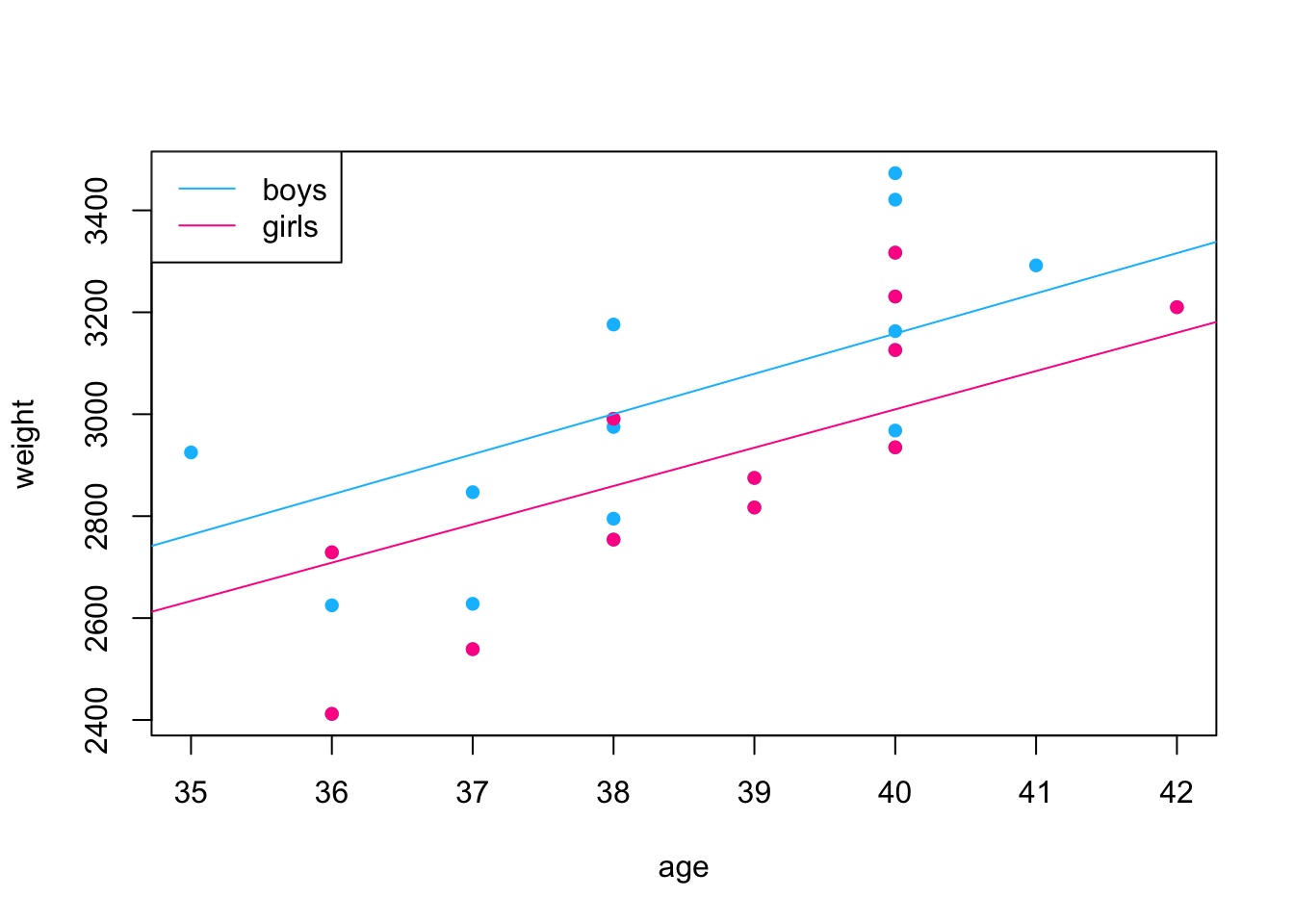

b_col <- "deepskyblue"
g_col <- "deeppink"
{
plot(f2, data = dtf, col = b_col, pch = 16)
points(dtf[dtf$gender == "girls",], col = g_col, pch = 16)
abline(lm2_boys, col = b_col)
abline(lm2_girls, col = g_col)
legend("topleft", c("boys", "girls"), lty = 1, col = c(b_col, g_col))
}

• The “R-squared” values is between 0 and 1. The lower end (closer to 0) indicate a poorly fitted model, the higher end (closer to 1) indicate a model of good fit.
• Adding gender to the model does improve the quality of the fit.

16.3 Non-linear models

16.3.1 Transformation

The Indometh dataset contains plasma concentration data of 6 subjects of indometacin, which was published in Kwan, Breault, Umbenhauer, McMahon and Duggan (1976) Kinetics of Indomethacin absorption, elimination, and enterohepatic circulation in man. Journal of Pharmacokinetics and Biopharmaceutics 4, 255–280.

Let’s first inspect the dataset:

# inspect the dataset
names(Indometh)

[1] "Subject" "time"    "conc"   

summary(Indometh)

 Subject      time            conc       
 1:11    Min.   :0.250   Min.   :0.0500  
 4:11    1st Qu.:0.750   1st Qu.:0.1100  
 2:11    Median :2.000   Median :0.3400  
 5:11    Mean   :2.886   Mean   :0.5918  
 6:11    3rd Qu.:5.000   3rd Qu.:0.8325  
 3:11    Max.   :8.000   Max.   :2.7200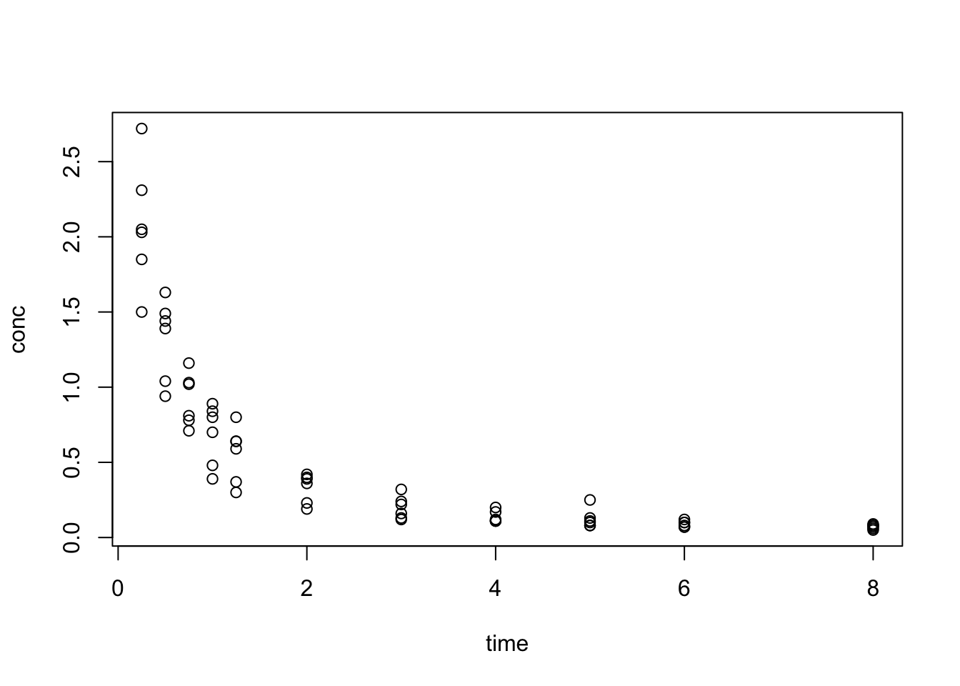  

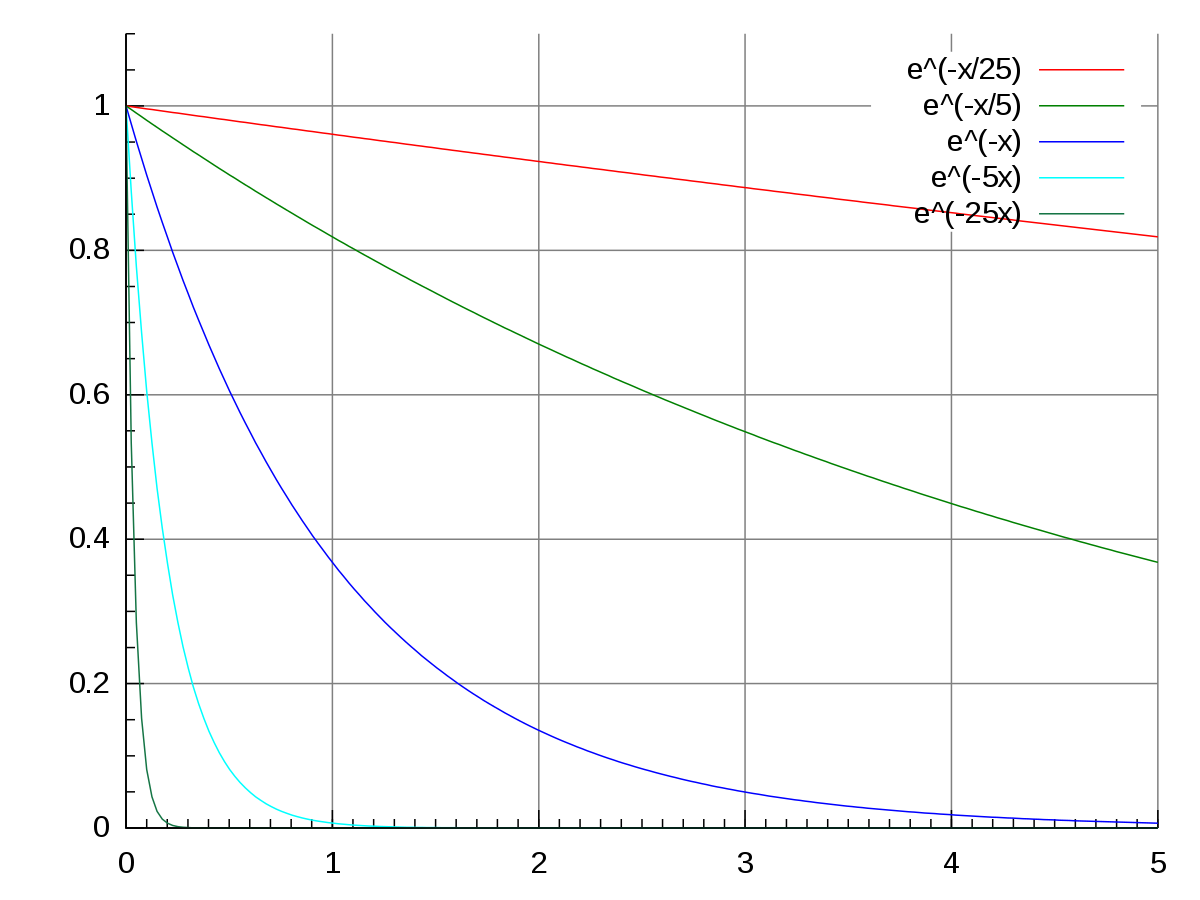
plot(conc ~ time, data = Indometh)

We see that data resembles the pattern of exponential decay:

image source

Therefore we transform conc with log() and get a linear regression fit:

\(log(conc) = b + a \times time\)

idm <- lm(log(conc) ~ time, data = Indometh)
summary(idm)

Call:
lm(formula = log(conc) ~ time, data = Indometh)

Residuals:
    Min      1Q  Median      3Q     Max 
-0.9558 -0.2940 -0.0206  0.3528  1.0125 

Coefficients:
            Estimate Std. Error t value Pr(>|t|)    
(Intercept)  0.09288    0.09337   0.995    0.324    
time        -0.41910    0.02468 -16.982   <2e-16 ***
---
Signif. codes:  0 '***' 0.001 '**' 0.01 '*' 0.05 '.' 0.1 ' ' 1

Residual standard error: 0.4904 on 64 degrees of freedom
Multiple R-squared:  0.8184,    Adjusted R-squared:  0.8155 
F-statistic: 288.4 on 1 and 64 DF,  p-value: < 2.2e-16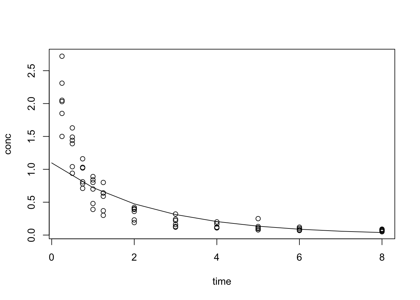

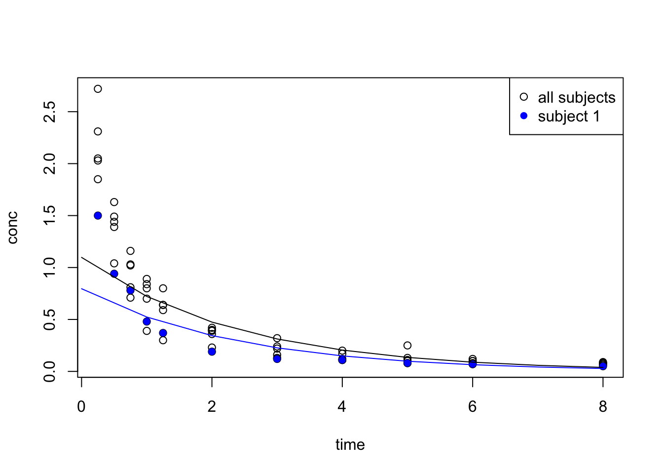
t <- 0:8
{
plot(conc ~ time, data = Indometh)
lines(
  x = t,
  y = exp(predict(idm, data.frame(time = t))) # note we need exp() to transform y back
)
}

Pick one subject for fitting:

Indometh_1 <- Indometh[Indometh$Subject == 1,]
idm_1 <- lm(log(conc) ~ time, data = Indometh_1)
summary(idm_1)

Call:
lm(formula = log(conc) ~ time, data = Indometh_1)

Residuals:
     Min       1Q   Median       3Q      Max 
-0.63614 -0.27362 -0.08709  0.33472  0.73837 

Coefficients:
            Estimate Std. Error t value Pr(>|t|)    
(Intercept) -0.22825    0.22407  -1.019    0.335    
time        -0.41862    0.05923  -7.068 5.87e-05 ***
---
Signif. codes:  0 '***' 0.001 '**' 0.01 '*' 0.05 '.' 0.1 ' ' 1

Residual standard error: 0.4804 on 9 degrees of freedom
Multiple R-squared:  0.8473,    Adjusted R-squared:  0.8304 
F-statistic: 49.96 on 1 and 9 DF,  p-value: 5.869e-05

{
t <- 0:8
plot(conc ~ time, data = Indometh)
points(conc ~ time, data = Indometh_1, pch = 16, col = "blue")
lines(
  x = t,
  y = exp(predict(idm_1, data.frame(time = t))),
  col = "blue"
)
lines(
  x = t,
  y = exp(predict(idm, data.frame(time = t))),
  col = "black"
)
legend("topright", legend = c("all subjects", "subject 1"), pch = c(1, 16), col = c("black", "blue") )
}

16.3.2 nls

We now further our search with an nls (non-linear least squares) regression search.

We fitted with lm with a transformed conc:

• \(log(conc) = b + a \times time\)
• b estimated at 0.09288
• a estimated at -0.41910

Transform the formula back to exponential form: \(conc = exp(b + a \times time)\) –> \(conc = exp(b) \times exp(a \times time)\)

A standard exponential growth function: \(P(t) = P_{0} \times exp(r \times t)\)

We take the result from lm as starting

p0_init <- exp(coefficients(idm)[1])
r_init  <- coefficients(idm)[2]

init <- list(p0 = unname(p0_init), r = unname(r_init))
init

$p0
[1] 1.097336

$r
[1] -0.4191029

idm_nls <- nls(conc ~ p0 * exp(r * time), data = Indometh, start = init)
summary(idm_nls)

Formula: conc ~ p0 * exp(r * time)

Parameters:
   Estimate Std. Error t value Pr(>|t|)    
p0  2.77706    0.15379   18.06   <2e-16 ***
r  -1.35038    0.09938  -13.59   <2e-16 ***
---
Signif. codes:  0 '***' 0.001 '**' 0.01 '*' 0.05 '.' 0.1 ' ' 1

Residual standard error: 0.2001 on 64 degrees of freedom

Number of iterations to convergence: 9 
Achieved convergence tolerance: 4.283e-06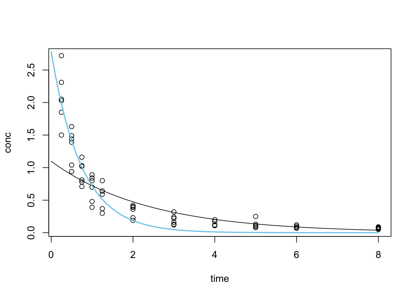

{
t <- seq(0, 8, by = 0.1)
plot(conc ~ time, data = Indometh)
lines(
  x = t,
  y = exp(predict(idm, data.frame(time = t))),
  col = "black"
)
lines(
  x = t,
  y = predict(idm_nls, data.frame(time = t)),
  col = "skyblue",
  lwd = 2
)
}

residuals(idm)
residuals(idm_nls)

sum(residuals(idm)^2)
sum(residuals(idm_nls)^2)

16.4 Optimisation with optim

Observing the fitted model from nls we see that the fitting is done in iterations until a convergence tolerance is met. This type of search is often applied when the optimal solution (the best fit curve) isn’t obvious and the search space is also big enough that it is (computationally) impossible to try all combinations of parameter values.

This class of problem, when generalised, is referred to as optimisation problems. optim is R’s general-purpose optimisation function.

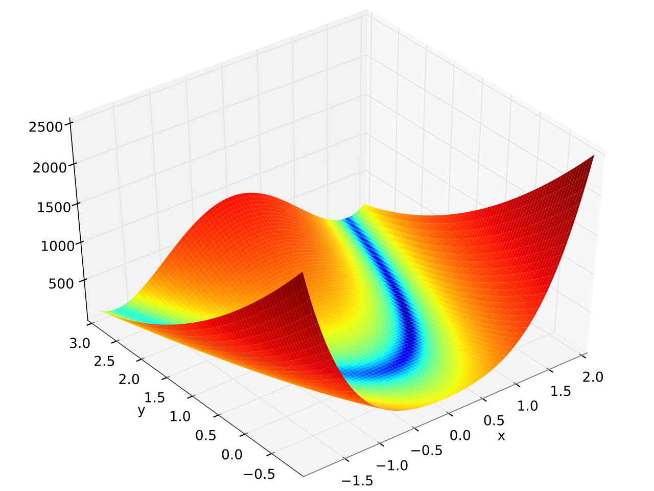
The Rosenbrock function is a non-convex function with the definition:

\(f(x, y) = (a - x)^2 + b(y-x^2)^2\)

The global minimum is at \((x, y) = (a, a^2)\) where \(f(x, y) = 0\)

image source

a <- 2
b <- 100
fr <- function(x) {   # Rosenbrock Banana function
    x1 <- x[1]
    x2 <- x[2]
    (a - x1)^2 + b * (x2 - x1 * x1)^2
}
optim(c(-1.2, 1), fr)

$par
[1] 2.000267 4.001077

$value
[1] 7.874009e-08

$counts
function gradient 
     265       NA 

$convergence
[1] 0

$message
NULL

See Test functions for optimisation for more functions like the Rosenbrock Banana function.

Exercises

E7.1

In our example using the WorldPhones dataset, we built a mathematical model assuming the number of new phones per year is a constant. What if we assume that the rate of change is constant, rather than the quantity? i.e. the number of phones has a constant year on year change rate of \(r\) such that:

\[n_{a+n} = n_{a}*(1+r)^{n}\]

1. Modify the mathematical model we implemented in the lecture with this new assumption.
2. Compare the results between these two different assumptions with a plot

E7.2

We talked about how linear interpolation can be done with approxfun during the lecture. But we only talked about how values are interpolated between the extremes of the dataset. What if we need values outside of these bounds? (Tip: Read the documentation on approxfun)

E7.3

During the lecture, we used the following code to demonstrate how an additional data point can change the result of polynomial interpolations. Modify the code to demonstrate how changes in data point values (in this case a new value for y8) can also affect the interpolation result.

set.seed(1)
x <- 1:10
y <- rnorm(10)
f <- splinefun(x, y)
x_extra <- 7.5
y_extra <- 0
f2 <- splinefun(c(x, x_extra), c(y, y_extra))

y8_new <- rnorm(1) # new value for y[8]

{
curve(f(x), 1, 10)
points(x, y)
# par(new = TRUE)
x2 <- seq(1, 10, by = 0.1)
y2 <- f2(x2)
lines(x2, y2, col = "red")
points(x_extra, y_extra, col = "red", pch = 16)
}

E7.4

Perform linear regression on R base’s built-in cars dataset.

E7.5

Perform linear regression on the anscombe dataset

E7.6

Use optim to find the minimum of the Golstein-Price function.