5 Environments
Environments consist of a frame, or collection of named objects, and a pointer to an enclosing environment. The most common example is the frame of variables local to a function call; its enclosure is the environment where the function was defined (unless changed subsequently). The enclosing environment is distinguished from the parent frame: the latter (returned by parent.frame) refers to the environment of the caller of a function.
Recommended readings:
5.1 .GlobalEnv
The global environment is the workspace where you interact with R. When you type an expression in the console, it is evaluated in the global environment. When you create a variable or a function, it is stored in the global environment. The global environment is also the top-level environment of the search path.
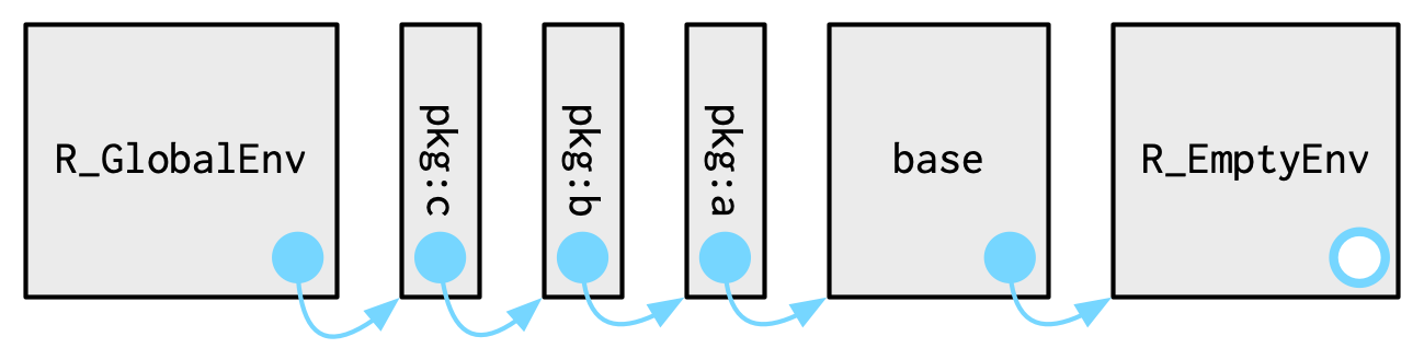
When a function is called, the R interpreter searches the implementation of the function along the search path
Once a new package is attached, it is added to the top of the search path, just behind GlobalEnv:
5.2 Create an environment
new.env, creates a new environmentls, returns a vector of all object (function and variable) names in an environment.rm, removes objects from a specified environment
ls gives information about what’s available in a package
5.3 Parent
Different environments can be linked together by setting the parent environment of one environment to another. When looking for an object, R will first look in the current environment, and if it doesn’t find it, it will look in the parent environment, and so on until it reaches the empty environment.
ftl <- function(x) { #"top level function"
  return(x * 2)
}

e1 <- new.env()
e2 <- new.env(parent = e1)
assign("a", 3, envir = e1)
ls(e1)
ls(e2)
exists("a", envir = e2)   # this succeeds by inheritance
exists("a", envir = e2, inherits = FALSE)
is.null(e2$a)
exists("ftl", envir = e2) # this succeeds by inheritance
exists("ftl", envir = e2, inherits = FALSE)
5.4 .with
withcan be used with both environments and list data structures that we will see in the next lecture